Bias-Variance User Guide
Motivation
Statistical Bias vs. “Fairness”
For this user guide and associated submodule, we are referring to statistical bias rather than the “fairness” type of bias.
Why should we care about bias and variance?
Bias and variance are two indicators of model performance and together represent two-thirds of model error (the remaining one-third is irreducible “noise” error that comes from the data set itself). We can define bias and variance as follows by training a model with multiple bootstrap sampled training sets, resulting in multiple instances of the model.
Typically, a model with high bias is “underfit” and a model with high variance is “overfit,” but keep in mind this is not always the case and there can be many reasons why a model has high bias or high variance. An “underfit” model is oversimplified and performs poorly on the training data, whereas an “overfit” model sticks too closely to the training data and performs poorly on unseen examples. See Scikit-Learn’s Underfitting vs. Overfitting for a clear example of an “underfit” model vs. an “overfit” model.
There is a concept known as the “bias-variance tradeoff” that describes the relationship between high bias and high variance in a model. Our ultimate goal here is to find the ideal balance where both bias and variance is at a minimum. It is also important from a business problem standpoint on whether the model error that we are unable to reduce should favor bias or variance.
Visualize Bias and Variance With Examples
In order to easily understand the concepts of bias and variance, we will show four different examples of models for each of the high and low bias and variance combinations. These are extreme and engineered cases for the purpose of clearly seeing the bias/variance.
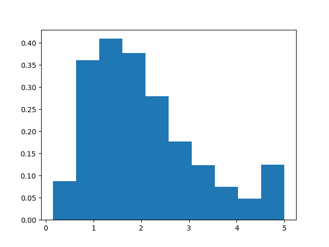
Before we begin, let’s take a look at the distribution of the labels. Notice that the majority of label values are around 1 and 2, and much less around 5.
First we have a model with high bias and low variance. We artificially introduce bias to the model by adding 10 to every training label, but leaving the test labels as is. Given that values of greater than 5 in the entire label set are considered outliers, we are fitting the model against outliers.
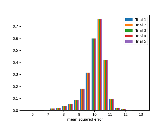
Five sets of mean squared error results from the test set from the five bootstrap sample trainings of the model. Notice the model error is very consistent among the trials and is not centered around 0.
Next we have a model with low bias and high variance. We simulate this by introducing 8 random “noise” features to the data set. We also reduce the size of the training set and train a neural network over a low number of epochs.
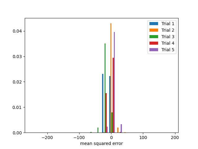
Five sets of mean squared error results from the test set from the five bootstrap sample trainings of the model. Notice the model error has different distributions among the trials and centers mainly around 0.
Next we have a model with high bias and high variance. We simulate through a combination of the techniques from the high bias low variance example and the low bias high variance example and train another neural network.
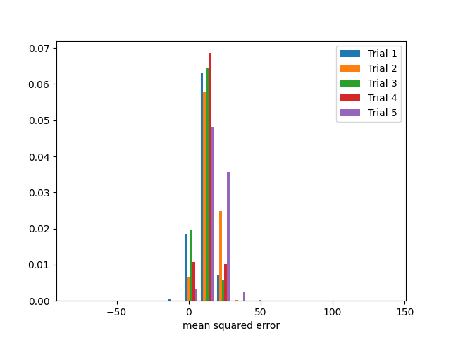
Five sets of mean squared error results from the test set from the five bootstrap sample trainings of the model. Notice the model error has different distributions among the trials and is not centered around 0.
Finally we have a model with low bias and low variance. This is a simple linear regression model with no modifications to the training or test labels.

Five sets of mean squared error results from the test set from the five bootstrap sample trainings of the model. Notice the model error is very consistent among the trials and centers mainly around 0.
Bias-Variance Decomposition
There are formulas for breaking down total model error into three parts: bias, variance, and noise. This can be applied to both regression problem loss functions (mean squared error) and classification problem loss functions (0-1 loss). In a paper by Pedro Domingos, a method of unified decomposition was proposed for both types of problems [Dom00].
First lets define \(y\) as a single prediction, \(D\) as the set of training sets used to train the models, \(Y\) as the set of predictions from the models trained on \(D\), and a loss function \(L\) that calculates the error between our prediction \(y\) and the correct prediction. The main prediction \(y_m\) is the smallest average loss for a prediction when compared to the set of predictions \(Y\). The main prediction is the mean of \(Y\) for mean squared error and the mode of \(Y\) for 0-1 loss [Dom00].
Bias can now be defined for a single example \(x\) over the set of models trained on \(D\) as the loss calculated between the main prediction \(y_m\) and the correct prediction \(y_*\) [Dom00].
Variance can now be defined for a single example \(x\) over the set of models trained on \(D\) as the average loss calculated between all predictions and the main prediction \(y_m\) [Dom00].
We will need to take the average of the bias over all examples as \(E_x[B(x)]\) and the average of the variance over all examples as \(E_x[V(x)]\) [Dom00].
With \(N(x)\) representing the irreducible error from observation noise, we can decompose the average expected loss as [Dom00]
In other words, the average loss over all examples is equal to the noise plus the average bias plus the net variance (the \(c\) factor included with the variance when calculating average variance gives us the net variance).
Note
We are generalizing the actual value of \(N(x)\), as the Model Validation Toolkit’s implementation of bias-variance decomposition does not include noise in the average expected loss. This noise represents error in the actual data and not error related to the model itself. If you would like to dive deeper into the noise representation, please consult the Pedro Domingos paper.
For mean squared loss functions, \(c = 1\), meaning that average variance is equal to net variance.
For zero-one loss functions, \(c = 1\) when \(y_m = y_*\) otherwise \(c = -P_D(y = y_* | y != y_m)\). [Dom00] In other words, \(c\) is 1 when the main prediction is the correct prediction. If the main prediction is not the correct prediction, then \(c\) is equal to the probability of a single prediction being the correct prediction given that the single prediction is not the main prediction.
Usage
bias_variance_compute() will return the average loss, average bias, average
variance, and net variance for an estimator trained and tested over a specified number
of training sets. This was inspired and modeled after Sebastian Raschka’s
bias_variance_decomp
function [Ras23].
We use the bootstrapping
method to produce our sets of training data from the original training set. By default
it will use mean squared error as the loss function, but it will accept the following
functions for calculating loss.
bias_variance_mse()for mean squared errorbias_variance_0_1_loss()for 0-1 loss
Since bias_variance_compute() trains an estimator over multiple iterations, it also
expects the estimator to be wrapped in a class that extends the
estimators.EstimatorWrapper class, which provides fit and predict methods
that not all estimator implementations conform to. The following estimator wrappers are
provided.
bias_variance_compute() works well for smaller data sets and less complex models, but what
happens when you have a very large set of data, a very complex model, or both?
bias_variance_compute_parallel() does the same calculation, but leverages Ray for parallelization of bootstrapping, training, and predicting.
This allows for faster calculations using computations over a distributed architecture.
Cem Anil, James Lucas, and Roger Grosse. Sorting out lipschitz function approximation. In International Conference on Machine Learning, 291–301. PMLR, 2019.
Martin Arjovsky, Soumith Chintala, and Léon Bottou. Wasserstein gan. arXiv preprint arXiv:1701.07875, 2017.
Marc G Bellemare, Ivo Danihelka, Will Dabney, Shakir Mohamed, Balaji Lakshminarayanan, Stephan Hoyer, and Rémi Munos. The cramer distance as a solution to biased wasserstein gradients. arXiv preprint arXiv:1705.10743, 2017.
Imre Csiszár, Paul C Shields, and others. Information theory and statistics: a tutorial. Foundations and Trends® in Communications and Information Theory, 1(4):417–528, 2004.
Pedro Domingos. A unified bias-variance decomposition and its applications. Technical Report, University of Washington, Seattle, WA, January 2000. URL: https://homes.cs.washington.edu/~pedrod/papers/mlc00a.pdf.
Arthur Gretton, Karsten M Borgwardt, Malte J Rasch, Bernhard Schölkopf, and Alexander Smola. A kernel two-sample test. Journal of Machine Learning Research, 13(Mar):723–773, 2012.
Ishaan Gulrajani, Faruk Ahmed, Martin Arjovsky, Vincent Dumoulin, and Aaron C Courville. Improved training of wasserstein gans. In Advances in neural information processing systems, 5767–5777. 2017.
Vincent Herrmann. Wasserstein gan and the kantorovich-rubinstein duality. February 2017. URL: https://vincentherrmann.github.io/blog/wasserstein/.
Sobol’ IM. Sensitivity estimates for nonlinear mathematical models. Math. Model. Comput. Exp, 1(4):407–414, 1993.
Jianhua Lin. Divergence measures based on the shannon entropy. IEEE Transactions on Information theory, 37(1):145–151, 1991.
XuanLong Nguyen, Martin J Wainwright, and Michael I Jordan. Estimating divergence functionals and the likelihood ratio by convex risk minimization. IEEE Transactions on Information Theory, 56(11):5847–5861, 2010.
Sebastian Nowozin, Botond Cseke, and Ryota Tomioka. F-gan: training generative neural samplers using variational divergence minimization. In Advances in neural information processing systems, 271–279. 2016.
Sebastian Raschka. Bias_variance_decomp: bias-variance decomposition for classification and regression losses. 2014-2023. URL: https://rasbt.github.io/mlxtend/user_guide/evaluate/bias_variance_decomp/.
Andrea Saltelli, Marco Ratto, Terry Andres, Francesca Campolongo, Jessica Cariboni, Debora Gatelli, Michaela Saisana, and Stefano Tarantola. Global sensitivity analysis: the primer. John Wiley & Sons, 2008.
Ilya M Sobol. Global sensitivity indices for nonlinear mathematical models and their monte carlo estimates. Mathematics and computers in simulation, 55(1-3):271–280, 2001.
Bharath K Sriperumbudur, Kenji Fukumizu, Arthur Gretton, Bernhard Schölkopf, and Gert RG Lanckriet. On integral probability metrics,\phi-divergences and binary classification. arXiv preprint arXiv:0901.2698, 2009.
Joel Aaron Tropp. Topics in sparse approximation. PhD thesis, University of Texas at Austin, 2004.
Geoffrey I Webb, Roy Hyde, Hong Cao, Hai Long Nguyen, and Francois Petitjean. Characterizing concept drift. Data Mining and Knowledge Discovery, 30(4):964–994, 2016.
Yihong Wu. Variational representation, hcr and cr lower bounds. February 2016. URL: http://www.stat.yale.edu/~yw562/teaching/598/lec06.pdf.