Thresholding User Guide
Motivation
Let’s say you’re monitoring some process for alerts. Maybe it’s model performance. Maybe it’s model drift. In any case, let’s say you have a score that increases with the likelihood that you have something wrong that needs to be investigated. You still need to decide whether to actually launch an investigation or not for each of these scores. This is known as thresholding. But where to put the threshold? Set it too high and you’ll miss important alerts. Set it too low and you’ll be flooded with noise. This module comes with tools and techniques to experimentally determine where to set your threshold given your tolerance for noise.
How?
Let’s say the scores associated with good alerts looks like this.
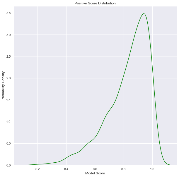
Moreover, scores associated with negative alerts look like this.

Clearly the likelihood of finding a good alert increases with model score, but any choice will imply a trade off between true/false positive/negatives. In general, you need to decide on a utility function of true/false positive/negatives.
The utility function would increase with true positives and/or true negatives, and decrease with false positives and/or false negatives. A risk averse utility function is shown above with a 20 fold preference of avoiding false negatives to false positives. In general, we will assume the utility function is a proportion of true/false positive/negatives in a data set. In this sense, the utility function is a function of a categorical distribution over true/false positives/negatives.
Now that we have a utility function, and a sample of positive and negative alert scores, we can plot a utility function as a function of threshold.
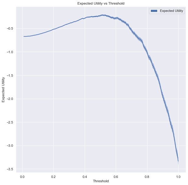
Expected utility as a function of threshold (solid) and 50% credible interval (shaded region).
Note that we don’t actually have the true distribution of positive and negative scores in practice. Rather, we have examples. If we only had 4 positive scores and 4 negative scores, we cannot be very certain of its results. More on this in the credibility user guide. We model the distribution of true/false positive/negatives as a Dirichlet-multinomial distribution with a maximum entropy prior.
This shows a particularly apparent peak in utility, but only after (in this case) a few thousand example scores. In practice, we could well be starting with no examples and building up our knowledge as we go. To make things worse, we will only find out if an alert was good or not if we investigate it. Anything that falls below our threshold forever remains unlabeled. We developed a specific algorithm to tackle this problem that we call adaptive thresholding.
Adaptive Thresholding
We face a classic exploitation/exploration dilemma. We can either choose to exploit the information we have so far about positive and negative score distributions to set a threshold or explore what may lie below that threshold by labeling whatever comes in next. Unfortunately, the labels obtained from scores greater than a threshold chosen at the time pose a challenge in that they yield heavily biased estimates of positive and negative score distributions (since they don’t include anything below the threshold set at the time). We have not found a good way to compensate for that bias in practice. Rather, we must switch between an optimally set threshold and labeling whatever comes next. This produces a series of unbiased labels.
Our adaptive thresholding algorithm seeks to balance the opportunity cost of labeling data with the utility gained over subsequent rounds with the change in threshold. Each score with an unbiased label is a potential threshold. For each of those options, we sample a possible distribution of true/false positives/negatives (with a Dirichlet-multinomial distribution with a maximum entropy prior) using the other unbiased labels. Utilities are calculated for each sampled distribution for true/false positives/negatives. The highest utility is noted as well as the utility of setting the threshold to 0 (exploration). Next this process is repeated using all but the most recent unbiased label. We locate the optimal threshold computed using all but the most recent unbiased label, and then compute the utility of that threshold using the utilities calculated using all unbiased labels. The difference between this utility and the utility of the true optimal threshold is the expected utility gained from the last round of exploration. This expected utility gained per round times the number of rounds since the last round of exploration is the net utility gained since the last round of experimentation. Meanwhile the difference between the utility of the true optimal threshold and the utility of exploration is the opportunity cost of exploration. When the net utility gained exceeds the opportunity cost of exploration, exploration is chosen over exploitation.
Note that we stochastically sample utilities at the score associated with each unbiased label at each round. This is necessary to prevent deadlocks in which the optimal threshold is identical before and after experimentation, leaving the expected utility gained per round 0 forever (thus ending any possibility of subsequent rounds of exploration). Rather, exploration is chosen according to the probability that net utility gained has in fact caught up with the opportunity cost of the last round of exploration.
However, as we gain a more accurate picture of the distribution of positive and negative scores, we make smaller changes to our best guess at the location of the optimal threshold after exploration. As a result, the expected utility gained per round of exploitation will gradually decrease over time, and we will need more and more rounds of exploitation to make up for the opportunity cost of exploration (shown below).
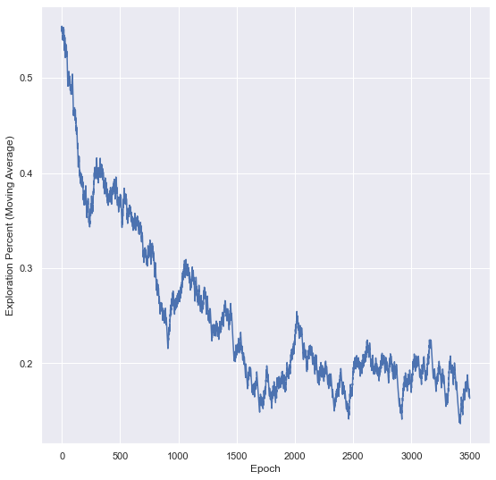
Probability of chosing exploration decreases from about 45% at the beginning to about 5% after 3600 rounds.
Cem Anil, James Lucas, and Roger Grosse. Sorting out lipschitz function approximation. In International Conference on Machine Learning, 291–301. PMLR, 2019.
Martin Arjovsky, Soumith Chintala, and Léon Bottou. Wasserstein gan. arXiv preprint arXiv:1701.07875, 2017.
Marc G Bellemare, Ivo Danihelka, Will Dabney, Shakir Mohamed, Balaji Lakshminarayanan, Stephan Hoyer, and Rémi Munos. The cramer distance as a solution to biased wasserstein gradients. arXiv preprint arXiv:1705.10743, 2017.
Imre Csiszár, Paul C Shields, and others. Information theory and statistics: a tutorial. Foundations and Trends® in Communications and Information Theory, 1(4):417–528, 2004.
Pedro Domingos. A unified bias-variance decomposition and its applications. Technical Report, University of Washington, Seattle, WA, January 2000. URL: https://homes.cs.washington.edu/~pedrod/papers/mlc00a.pdf.
Arthur Gretton, Karsten M Borgwardt, Malte J Rasch, Bernhard Schölkopf, and Alexander Smola. A kernel two-sample test. Journal of Machine Learning Research, 13(Mar):723–773, 2012.
Ishaan Gulrajani, Faruk Ahmed, Martin Arjovsky, Vincent Dumoulin, and Aaron C Courville. Improved training of wasserstein gans. In Advances in neural information processing systems, 5767–5777. 2017.
Vincent Herrmann. Wasserstein gan and the kantorovich-rubinstein duality. February 2017. URL: https://vincentherrmann.github.io/blog/wasserstein/.
Sobol’ IM. Sensitivity estimates for nonlinear mathematical models. Math. Model. Comput. Exp, 1(4):407–414, 1993.
Jianhua Lin. Divergence measures based on the shannon entropy. IEEE Transactions on Information theory, 37(1):145–151, 1991.
XuanLong Nguyen, Martin J Wainwright, and Michael I Jordan. Estimating divergence functionals and the likelihood ratio by convex risk minimization. IEEE Transactions on Information Theory, 56(11):5847–5861, 2010.
Sebastian Nowozin, Botond Cseke, and Ryota Tomioka. F-gan: training generative neural samplers using variational divergence minimization. In Advances in neural information processing systems, 271–279. 2016.
Sebastian Raschka. Bias_variance_decomp: bias-variance decomposition for classification and regression losses. 2014-2023. URL: https://rasbt.github.io/mlxtend/user_guide/evaluate/bias_variance_decomp/.
Andrea Saltelli, Marco Ratto, Terry Andres, Francesca Campolongo, Jessica Cariboni, Debora Gatelli, Michaela Saisana, and Stefano Tarantola. Global sensitivity analysis: the primer. John Wiley & Sons, 2008.
Ilya M Sobol. Global sensitivity indices for nonlinear mathematical models and their monte carlo estimates. Mathematics and computers in simulation, 55(1-3):271–280, 2001.
Bharath K Sriperumbudur, Kenji Fukumizu, Arthur Gretton, Bernhard Schölkopf, and Gert RG Lanckriet. On integral probability metrics,\phi-divergences and binary classification. arXiv preprint arXiv:0901.2698, 2009.
Joel Aaron Tropp. Topics in sparse approximation. PhD thesis, University of Texas at Austin, 2004.
Geoffrey I Webb, Roy Hyde, Hong Cao, Hai Long Nguyen, and Francois Petitjean. Characterizing concept drift. Data Mining and Knowledge Discovery, 30(4):964–994, 2016.
Yihong Wu. Variational representation, hcr and cr lower bounds. February 2016. URL: http://www.stat.yale.edu/~yw562/teaching/598/lec06.pdf.