Notes on Using Divergence Functions

The mvtk.supervisor.divergence contains several functions that compute total variation between two data distributions. However, these functions have very different mechanisms for arriving at total variation. Some functions, such as calc_tv use a neural network under the hood, while others such as calc_tv_knn use a different mechanism to arrive at the range of values to inform on whether two distributions are more similar or not. Because of these differences, there functions are often best suited for different circumstances, be it data size, computational resources, or accuracy requirements. This notebook provides a guide to when and how to use the functions.

import numpy as np
import warnings
from IPython.display import display
from ipywidgets import HTML
warnings.filterwarnings('ignore')
from mvtk.supervisor.divergence import calc_tv, calc_tv_knn, calc_tv_density, calc_tv_mle, calc_kl_mle, calc_hl
from mvtk.supervisor.utils import column_indexes

Data Types

The algorithms underneath the divergence functions all operate on numpy arrays. A divergence function compares a sample_a vs a sample_b, where a sample is either an array

def divergence_function(sample_a, sample_b, **kwargs):
    algorithm

OR a list of arrays

def divergence_function([sample_a], [sample_b], **kwargs):
    algorithm

The functions that accept lists allow you to test one list of batches against another list of batches. For example,

sample_a = [batch1, batch2, batch3]
sample_b = [[batch5, batch6]

This will compare the average of the distributions that generated batch1, batch2, and batch3 to the average of the distributions that generated batch4 and batch5. You can just use singletons to compare batch1 to batch2, i.e.

sample_a = [batch1]
sample_b = [batch2]

For the divergence functions that you intend to use, you should check the documentation as to whether it accepts lists or arrays.

Using Dataframes

Pandas dataframes are a perfect input source for the divergence functions. The underlying storage for dataframes are numpy arrays on which all divergence functions can operate.

If your data is in Pyspark dataframes then you either convert to pandas dataframes, or numpy arrays.

import pandas as pd
df = pd.DataFrame({'weight': np.random.uniform(1, 100, size=(10000)),
                  'colors': np.random.choice(['red', 'blue', 'green', 'yellow'], p=[0.2, 0.3, 0.3, 0.2])})
df.head(3)

	weight	colors
0	79.360725	green
1	92.373537	green
2	91.021177	green

Create Data Distributions

For data, we will create datasets drawn from different distributions. We will use about a million rows, and about 100 columns.

Each row in a dataset becomes a training example to be used in the neural network that calculates the divergence. If you have too few rows, then the divergence value will not be calculated accurately, and in practice will be close to zero.

ROWS, COLUMNS = 1000000, 10
DATA_SHAPE = ROWS, COLUMNS

samples = dict()
uniform_a   = samples['uniform_a']   = np.random.uniform(1, 100, size=DATA_SHAPE)
uniform_b   = samples['uniform_b']   = np.random.uniform(1, 100, size=DATA_SHAPE)
beta_a      = samples['beta_a']      = np.random.beta(0.2, 0.9, size=DATA_SHAPE)
chisquare_a = samples['chisquare_a'] = np.random.chisquare(2,DATA_SHAPE)
ones        = samples['ones']        = np.ones(DATA_SHAPE)

funcs = {'calc_tv': calc_tv}

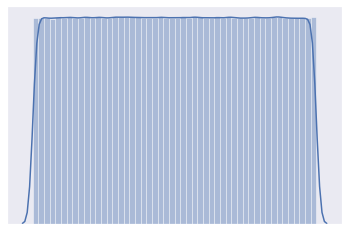
Visualizing the distributions

Let’s visualize each of our probability distributions. In this case, each of the COLUMNS=10 features has exactly the same distribution and they are all independent of eachother, so the following function just lumps all of the samples together. In general, you would not want to do this!

import matplotlib.pyplot as plt
import matplotlib.style as style
import seaborn as sns; sns.set()

def distplot(series, title=None):
    if isinstance(series, pd.Series):
        series = series.values
    sns.distplot(series.ravel())
    plt.xticks([])
    plt.yticks([])
    plt.grid(False)
    if title:
        plt.title(title)

distplot(uniform_a)

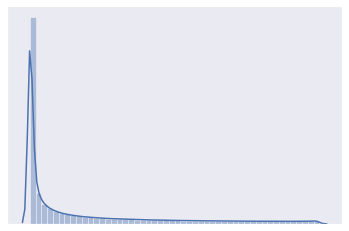
distplot(beta_a)

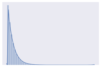
distplot(chisquare_a)

distplot(ones)

Calculating Total Variation

The main divergence functions calculate the total variation between distributions. However, there are very different ways to arrive at a range of 0-1 with 0 meaning no divergence, and 1 meaning total divergence. This presents users with different approaches with benefits that match different circumstances and dta sizes.

calc_tv

Computes the total variation between two distributions.

See https://en.wikipedia.org/wiki/Total_variation_distance_of_probability_measures It uses a neural network to calculate the total variation between distributions. Since it uses a neural network internally, it exposes some familar settings such as the num_epochs, num_batches etc. which you can tune for greater accuracy.

sample_distribution_p The first distribution

sample_distribution_q The second distribution

categorical_columns If using a dataframe, the categorical columns

num_epochs The number of epochs to train for

num_batches

Additionally, you can use model_generator_kwargs to set model_generator default **kwargs. Of particular importance are:

depth The number of layers of the neural network. Defaults to 3

width The size of the hidden layer

calc_tv(uniform_a, uniform_b)

0.0004881620407104492

If two distributions are different then the divergence will be close to one.

calc_tv(uniform_a, ones)

0.9995993375778198

You can get better accuracy by changing the default parameters - in this case num_epochs=16, num_batches=128, depth=2, width=32

calc_tv(uniform_a, ones, num_epochs=16, num_batches=128, model_generator_kwargs={'width': 32, 'depth': 2})

0.999308705329895

calc_tv(uniform_a, chisquare_a)

0.9999822974205017

calc_tv(uniform_a, [pd.DataFrame(chisquare_a), ones])

0.9989728927612305

calc_tv([uniform_a, ones],[chisquare_a])

0.5061822533607483

calc_hl

Calculate divergence using Hellinger distance.

See https://en.wikipedia.org/wiki/Hellinger_distance

sample_distribution_p The first distribution

sample_distribution_q The second distribution

Additionally, you can use model_generator_kwargs to set model_generator default **kwargs. Of particular importance are:

depth The number of layers of the neural network. Defaults to 3

width The size of the hidden layer

calc_hl(uniform_a, uniform_b)

0.0

calc_hl(uniform_a, chisquare_a)

0.0

calc_hl finds a significant divergence between the beta and chisquare distributions

calc_hl(beta_a, chisquare_a)

0.9981940472630377

calc_tv_knn

Computes the total variation between two distributions. Because it uses KNN which is a fairly simple algorithm it is often faster to compute that calc_tv. However, you will want to take care to set the function parameters based on your data dimensions in order for it to get the best accuracy.

sample_distribution_p The first distribution

sample_distribution_q The second distribution

bias

num_samples Number of subsamples to take from each distribution on which to construct kdtrees and otherwise make computations. Defaults to 2046

categorical_columns

k number of nearest neighbours. As a rule of thumb, you should multiply this by two with every dimension past one. Defaults to 128

Here is an example of using the default parameters for calc_tv_knn on similar distributions.

calc_tv_knn(uniform_a, uniform_b)

0.03465665858242252

In this example, calc_tv_knn picks up a divergence between the uniform and beta distributions

calc_tv_knn(uniform_a, beta_a, k=20)

0.8272527964149479

and between the uniform and chisquare distributions

calc_tv_knn(uniform_a, chisquare_a)

0.9306603225843605

KNN is an unbiased estimator and will sometimes overshoot.

calc_tv_knn(beta_a, chisquare_a)

1.20928344516188

One way to address this is to set the value of k neighbours to 2 * the number of dimensions. There are 10 columns so we set k to 20.

calc_tv_knn(beta_a, chisquare_a, k = 20)

1.1124090464149479

calc_tv_knn(beta_a, beta_a, k=20)

0.07457887528399548

Density Based Estimators

Density estimation is the problem of reconstructing the probability density function using a set of given data points.

calc_tv_density

calc_tv_density(uniform_a, uniform_b)

165011946.1532011

calc_tv_density(uniform_a, beta_a)

251557894.78209227

Handling Categorical Data

If your data is all categorical, then you would probably want to use calc_tv_mle.

For these examples, we will create categorical columns drawn from different distributions.

FRUITS, FRUIT_PROBS = ['apple', 'orange', 'plum', 'raspberry', 'blueberry'], [0.1, 0.3, 0.3, 0.25, 0.05]
assert sum(FRUIT_PROBS) ==1

raspberry_blast = np.random.choice(FRUITS,size=(1000000, 10), p=FRUIT_PROBS)
blueberry_blast = np.random.choice(FRUITS,size=(1000000, 10), p=FRUIT_PROBS)
plain_smoothie = np.random.choice(FRUITS, size=(1000000, 10))

calc_tv_mle

Computes the total variation between two distributions using histogram based density estimators. All columns are assumed to be categorical.

sample_distribution_p The first distribution

sample_distribution_q The second distribution

raspberry_blast[0]

array(['orange', 'apple', 'plum', 'plum', 'plum', 'plum', 'orange',
       'raspberry', 'plum', 'orange'], dtype='<U9')

The samples raspberry_blast and plain_smoothie have been drawn from different distributions and so we expect to see a high total variation.

calc_tv_mle(raspberry_blast, plain_smoothie)

0.9319870000000001

But the samples raspberry_blast and plain_smoothie have been drawn from similar distributions and so we expect to see lower total variation.

calc_tv_mle(raspberry_blast, blueberry_blast)

0.6263819999999999

calc_kl_mle

When the second distribution is zero when the first distribution is nonzero for categorical data, kl divergence will hit infinity. For histograms derived from high dimensional categorical data this becomes likely.

calc_kl_mle(raspberry_blast, plain_smoothie)

inf

Handling Mixed Data

If your data contains categorical columns, then you need to specify the indices of the categorical columns. To demonstrate this, we will create a dataframe with one categorical column and one numeric column, then compute the total variation.

NUM_ITEMS = 100000
inventory_a = pd.DataFrame({'fruits': np.random.choice(FRUITS,size=NUM_ITEMS, p=FRUIT_PROBS),
                          'weight': np.random.uniform(1, 100, size=NUM_ITEMS).tolist()})

inventory_b = pd.DataFrame({'fruits': np.random.choice(FRUITS,size=NUM_ITEMS),
                            'weight': np.random.beta(0.2, 0.9, size=NUM_ITEMS).tolist()})

inventory_a.head(4)

	fruits	weight
0	plum	9.043091
1	orange	82.114676
2	raspberry	31.065103
3	raspberry	64.049112

inventory_b.head(4)

	fruits	weight
0	plum	0.001619
1	plum	0.000238
2	raspberry	0.978383
3	orange	0.514946

Now we can use calc_tv_knn, setting k=4 since there are only two columns

calc_tv_knn(inventory_a, inventory_b, categorical_columns=[0], k=4)

0.664169492122229

If you use calc_tv_knn on the same data you get a lower value since it’s the same distribution

calc_tv_knn(inventory_a, inventory_a, categorical_columns=[0], k=4)

0.216708554622229