Interprenet User Guide
Motivation
Neural networks are generally difficult to interpret. While there are tools that can help to interpret certain types of neural networks such as image classifiers and language models, interpretation of neural networks that simply ingest tabular data and return a scalar value is generally limited to various measures of feature importance. This can be problematic as what makes a feature “important” can vary between use cases.
Rather than interpret a neural network as a black box, we seek to constrain neural network in ways we consider useful and interpretable. In particular, The interprenet module currently has two such constraints implemented:
Monotonicity
Lipschitz constraint
Monotonic functions either always increase or decrease with their arguments but never both. This is often an expected relationship between features and the model output. For example, we may believe that increasing blood pressure increases risk of cardiovascular disease. The exact relationship is not known, but we may believe that it is monotonic.
Lipschitz constraints constrain the maximum rate of change of the model. This can make the model arbitrarily robust against adversarial perturbations [ALG19].
How?
All constraints are currently implemented as weight constraints. While arbitrary weights are stored within each linear layer, the weights are transformed before application so the network can satisfy is prescribed constraints. Changes are backpropagated through this transformation. Monotonic increasing neural networks are implemented by taking the absolute value of weight matrices before applying them. When paired with a monotonically increasing activation (such as ReLU, Sigmoid, or Tanh), this ensures the gradient of the output with respect to any features is positive. This is sufficient to ensure monotonicity with respect to the features.
Lipschitz constraints are enforced by dividing each weight vector by its \(L^\infty\) norm as described in [ALG19]. This constrains the \(L^\infty\)-\(L^\infty\) operator norm of the weight matrix [Tro04]. Constraining the \(L^\infty\)-\(L^\infty\) operator norm of the weight matrix ensures every element of the jacobian of the linear layers is less than or equal to \(1\). Meanwhile, using activation functions with Lipschitz constants of \(1\) ensure the entire network is constrained to never have a slope greater than \(1\) for any of its features.
Different Constraints on Different Features
constrained_model() generates a neural network with one set of
constraints per feature. Constraints currently available are:
identity()(for no constraint)
Features are grouped by the set of constraints applied to them, and different constrained neural networks are generated for each group of features. The outputs of those neural networks are concatenated and fed into a final neural network constrained using all constraints applied to all features. Since constraints on weight matrices compose, they can be applied as a series of transformations on the weights before application.
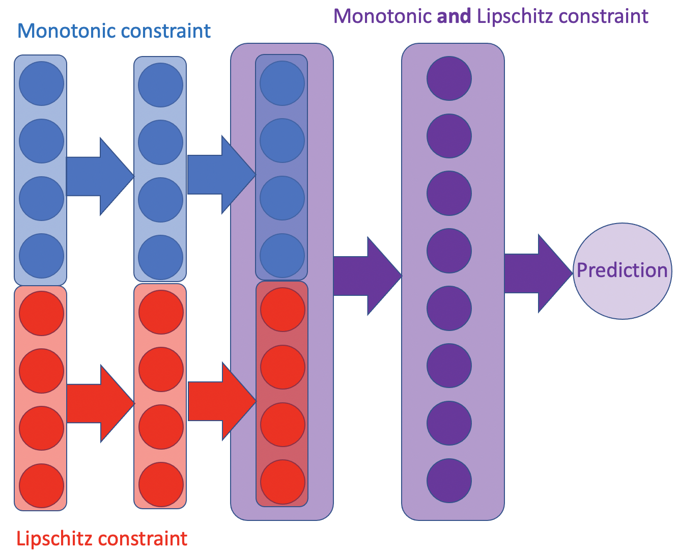
4 features with Lipschitz constraints and 4 features wtih monotonic constraints are fed to their respectively constrained neural networks. Intermediate outputs are concatenated and fed into a neural network with monotonic and lipschitz constraints.
We use the Sort function as a nonlinear activation as described in [ALG19]. The jacobian of this matrix is always a permutation matrix, which retains any Lipschitz and monotonicity constraints.
Preprocessing
Thus far, we have left out two important detail: How to constrain
the Lipschitz constant to be something other than \(1\), and how
to create monotonically decreasing networks. Both are a simple
matter of preprocessing. The preprocess argument (defaulting to
identity), specifies a function to be applied to the feature
vector before passing it to the neural network. For decreasing
monotonic constraints, multiply the respective features by
\(-1\). For a Lipschitz constant of \(L\), multiply the
respective features by \(L\).
Cem Anil, James Lucas, and Roger Grosse. Sorting out lipschitz function approximation. In International Conference on Machine Learning, 291–301. PMLR, 2019.
Martin Arjovsky, Soumith Chintala, and Léon Bottou. Wasserstein gan. arXiv preprint arXiv:1701.07875, 2017.
Marc G Bellemare, Ivo Danihelka, Will Dabney, Shakir Mohamed, Balaji Lakshminarayanan, Stephan Hoyer, and Rémi Munos. The cramer distance as a solution to biased wasserstein gradients. arXiv preprint arXiv:1705.10743, 2017.
Imre Csiszár, Paul C Shields, and others. Information theory and statistics: a tutorial. Foundations and Trends® in Communications and Information Theory, 1(4):417–528, 2004.
Pedro Domingos. A unified bias-variance decomposition and its applications. Technical Report, University of Washington, Seattle, WA, January 2000. URL: https://homes.cs.washington.edu/~pedrod/papers/mlc00a.pdf.
Arthur Gretton, Karsten M Borgwardt, Malte J Rasch, Bernhard Schölkopf, and Alexander Smola. A kernel two-sample test. Journal of Machine Learning Research, 13(Mar):723–773, 2012.
Ishaan Gulrajani, Faruk Ahmed, Martin Arjovsky, Vincent Dumoulin, and Aaron C Courville. Improved training of wasserstein gans. In Advances in neural information processing systems, 5767–5777. 2017.
Vincent Herrmann. Wasserstein gan and the kantorovich-rubinstein duality. February 2017. URL: https://vincentherrmann.github.io/blog/wasserstein/.
Sobol’ IM. Sensitivity estimates for nonlinear mathematical models. Math. Model. Comput. Exp, 1(4):407–414, 1993.
Jianhua Lin. Divergence measures based on the shannon entropy. IEEE Transactions on Information theory, 37(1):145–151, 1991.
XuanLong Nguyen, Martin J Wainwright, and Michael I Jordan. Estimating divergence functionals and the likelihood ratio by convex risk minimization. IEEE Transactions on Information Theory, 56(11):5847–5861, 2010.
Sebastian Nowozin, Botond Cseke, and Ryota Tomioka. F-gan: training generative neural samplers using variational divergence minimization. In Advances in neural information processing systems, 271–279. 2016.
Sebastian Raschka. Bias_variance_decomp: bias-variance decomposition for classification and regression losses. 2014-2023. URL: https://rasbt.github.io/mlxtend/user_guide/evaluate/bias_variance_decomp/.
Andrea Saltelli, Marco Ratto, Terry Andres, Francesca Campolongo, Jessica Cariboni, Debora Gatelli, Michaela Saisana, and Stefano Tarantola. Global sensitivity analysis: the primer. John Wiley & Sons, 2008.
Ilya M Sobol. Global sensitivity indices for nonlinear mathematical models and their monte carlo estimates. Mathematics and computers in simulation, 55(1-3):271–280, 2001.
Bharath K Sriperumbudur, Kenji Fukumizu, Arthur Gretton, Bernhard Schölkopf, and Gert RG Lanckriet. On integral probability metrics,\phi-divergences and binary classification. arXiv preprint arXiv:0901.2698, 2009.
Joel Aaron Tropp. Topics in sparse approximation. PhD thesis, University of Texas at Austin, 2004.
Geoffrey I Webb, Roy Hyde, Hong Cao, Hai Long Nguyen, and Francois Petitjean. Characterizing concept drift. Data Mining and Knowledge Discovery, 30(4):964–994, 2016.
Yihong Wu. Variational representation, hcr and cr lower bounds. February 2016. URL: http://www.stat.yale.edu/~yw562/teaching/598/lec06.pdf.