Supervisor User Guide
Motivation
My Model is Done!
OK, so your model is trained and ready to be put into a production pipeline. Models are, however, not like hard coded rules in the sense that they are not expected to work perfectly all the time. They are expected to work well most of the time. And just because a model was tested on a sample of data does not mean it will continue to be accurate forever.
Think of it this way, you want to predict human weight from height. You build a linear model from some demographics from a small US city that multiplies height by some number and adds another number, and is on average pretty accurate for predicting weight. Great! Now you put it into production, and it works fine. A few years later, a series of fast food chains opens up, and everyone in the town starts gaining weight. Your model becomes less accurate because the data you built it on is no longer a valid representation of the current population. This is why you need a monitoring system. It costs almost nothing to put one in place, and it’s the only way you’ll know if your model is still accurate over time.
How?
There are tons of ways to evaluate model performance, but they all require you to know what you wanted the model to say in hindsight. These metrics are typically used to assess accuracy during training and validation. Going back to our example, we could tell exactly the degree to which our linear weight from height model was degrading each year by measuring everyone’s weight and height each year. That’s fine if you don’t mind waiting to take measurements. In real life, there are lots of situations for which we get pretty fast feedback, and for those situations, it’s fine just to validate the model on new incoming data in the same manner that it was validated during training. However, there are also plenty of situations where this is not the case…
Divergence What?
Just as we can compare the data coming out of a model to ground truth, we can compare the data coming into the model to the training data. In the former case, we match up each prediction to the answer we wished in hindsight we had gotten, and summarize the results with any number of accuracy metrics. We can generally compare the inputs to the input data used to train the model. In this sense, we can ask questions like “Does this batch of inputs seem distributed like the training data?” and “Does this particular input look strange relative to what was used in the training data?” In the former case, your inputs generally arrive in batches. Maybe once a month you collect height data and run your model to compute weights. You can then ask does this month’s height distribution look similar to the height distribution of the training data? It may seem hard to quantify, and that’s because it is! Though it’s not impossible. There are a number of so called statistical divergences. They give a number that represents how similar two distributions are. For example, two identical Gaussians might get a score of 0, and a Gaussian paired with a uniform distribution might get a score of 0.4. Generally, a divergence will give its lowest possible score when the two distributions are the one and the same, and its highest possible value when they predict mutually exclusive outcomes (e.g. distribution one says a coin will always come up tails and distribution two says a coin will always come up heads). We can recommend and have implemented a few metrics in the Supervisor that have some other useful properties like symmetry (the number compare distribution one to distribution two is the same number computed from comparing distribution two to distribution one) and the triangle inequality (divergence of distribution one and two plus divergence of distribution two and three is less than or equal to divergence of distribution one and three). In math jargon, these extra properties make these divergences metrics which in turn means they have the same consistencies you would intuitively associate with a measure of distance. This makes plots much more meaningful because your intuition about distances holds when you look at a plot involving divergence metrics.
Divergences
Divergences are all about quantifying differences between two probability distributions. This is not just about a literal subtraction of one value from another, so much as coming up with a process that assigns a number that quantifies how different two (or more) probability distributions are. For example, the number might decrease as the two distributions approach being one and the same. Generally, the number will approach its maximum (which can be infinity!) when there exist no events that can be sampled from both distributions. For example, a coin that would always come up heads in the first distribution would always come up tails in the second distribution. In other words, they are singular.
A common and useful metric is called total variation. Total variation is defined as one half the average absolute difference between the two probability distributions being compared, \(p\) and \(q\) [Wu16].
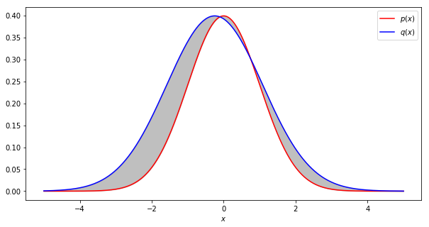
Total variation is one half the average absolute difference between two probability distributions (shown in grey).
By factoring out \(q(x)\) and applying the law of large numbers, this can be rewritten as
This is one example of what are generally known as an \(f\) (sometimes \(\phi\)) divergence. In the case of total divergence, \(f\left(\frac{q}{p}\right) = \frac{1}{2}\left\vert 1 - \frac{q}{p}\right\vert\). In general, \(f\) can be any convex function of \(\frac{p}{q}\) with its minimum at \(p=q\) (typically such that \(f(1)=0\)). This class of measures will produce a statistic that decreases as \(p\) approaches \(q\) [CsiszarS+04] [Wu16]. It is easy to see by the change of variables formula for probability density functions that this class of divergences encompasses every divergence that is invariant to coordinate transformations. There are many other commonly cited \(f\)-divergences, including Hellinger distance, Kullback–Leibler (KL) divergence, and Jensen-Shannon divergence [NCT16]. Jensen-Shannon divergence admits a natural generalization that measures the mutual distance of multiple probability distributions, and all of the divergences measured thus far are bounded between \(0\) and \(1\).
In general, not all \(f\) divergences are proper metrics. As a motivating example, consider KL-divergence:
Clearly, this divergence is not even symmetric with respect to \(p\) and \(q\). As it turns out, it does not obey the triangle inequality either. This is not always bad. The KL-divergence is a useful measure, and will increase as \(p\) and \(q\) become less similar. However, it lacks any intuitive sense of distance as plotted over time. For this reason, most analyses of concept drift prefer divergences that are proper metrics [WHC+16].
As we shall see, there are two ways to estimate \(f\)-divergences: with density estimators, and with variational methods.
Estimation with Density Estimators
The most intuitive approach to estimating f-divergences is with density estimation. This involves estimating \(p(x)\) and \(q(x)\) given a finite number of samples, and then plugging those estimates into the explicit formula for your f-divergence.
Here, \(\mathcal{X}\) is the shared sample space of \(p\) and \(q\). The simplest form of density estimator is a histogram, and the Supervisor not only provides common utilities for density estimator based estimates of \(f\)-divergences, but also can also construct histograms from raw data.
The following functions come with the Supervisor’s divergence module for estimating \(f\)-divergences by explicitly constructing histograms from raw samples.
Alternatively, if you chose to construct your own density estimates, you can use the following functions to calculate \(f\)-divergences from those.
Variational Estimation of \(f\)-divergences
Density estimation via histograms is straightforward, and indeed a gold standard of sorts, for categorical data. However, constructing histograms for real valued data requires binning, which tends to become increasingly inaccurate for high dimensional samples. Variational estimation, while only directly applicable to real valued data, is generally believed to scale better with the number of features [SFG+09] [NWJ10].
What are variational estimates? In general, variational methods refer to a problem involving finding a function that satisfies some optimization problem. In other words, if an ordinary optimization problem involves finding an optimal location in a finite dimensional coordinate system, variational problems involve finding optimal location in function space, which involves an uncountably infinite number of coordinates.
There are some clever tricks from convex analysis [Wu16] that can apply to \(f\)-divergences. We first define the convex conjugate as
The Fenchel–Moreau theorem states that if \(f\) is a proper convex function and lower semicontinuous, then \(f^{**}(g) = f(g)\).
This is true for a wide variety of useful functions \(f\) [NCT16]. Under these conditions, we have
If we let \(y=\frac{p(x)}{q(x)}\) for some point, \(x\), within the sample space of \(p\) (which is assumed to be the same as that of \(q\)),
, where the inequality follows from the definition of the supremum. Furthermore, if we tether \(g\) to that same sample, \(x\), in the form of \(g(x)\), we get
Multiplying both sides by \(q(x)\)
Integrating both sides over \(x\) drawn from the sample space, \(\mathcal{X}\),
Finally, we can apply the law of large numbers to turn integrals over probability density functions into expectations.
This final result shows that an \(f\)-divergence can be expressed as a function optimization problem. In this case, the right hand side of the inequality prescribes a loss function with which we use to find a function \(g(x)\). Specifically, the loss function used would be the negative of the right hand side. When the loss is minimized, the right hand side is maximized and the inequality approaches equality to the left hand side (i.e. the true \(f\)-divergence).
In practice, we can use a function approximator, such as a neural network to find \(g(x)\). This in fact yields an unbiased estimator of the gradient when trained via stochastic gradient descent [NCT16].
Note
It’s also worth noting the significance of \(g(x)\). Rather than approximating \(p(x)\) and \(q(x)\) individually, the model trained to approximate \(g(x)\) has learned the likelihood ratio, \(\frac{p(x)}{q(x)}\) [NWJ10].
Where we are able to invert \(f^{*\prime}\) when \(f^{*}\) is strictly convex, and therefore has a strictly monotonic derivative when differentiable.
The following functions come with the Supervisor’s divergence module for estimating \(f\)-divergences using variational methods.
Variational estimation is only applicable for numerically encoded data, and was found to work poorly for one hot encoded categorical data with large numbers of categories.
Hybrid Estimation
What if we have data that is partially categorical, and partially real valued? Are we just limited to binning the real valued data to effectively make the entire dataset categorical? As of the time of this writing, this seems to have generally been the case. The Supervisor team has, however, implemented an experimental hybrid approach just for you! Let’s return to the variational formalism.
Let’s say \(x\) had some categorical components, \(x_c\) and some real valued components, \(x_r\).
To effectively use \(x_c\) within our model for \(g(x_c, x_r)\), we may store a table of functions \(g_{x_c}(x_r)\) and simultaneously train them as minibatches are sampled. In this way, every unique combination of categorical variables, \(x_c\), specifies a model \(g_{x_c}\) that is trained using a respective \(x_r\). This requires storing and training as many models as there are unique combinations of categorical inputs within the given datasets. The performance of our hybrid approach will generally degrade linearly with the number of unique combinations of categorical inputs.
In general, any variational method for computing divergences supports hybrid
estimation using two techniques. The categorical_columns argument can be
used to specify the indices of categorical features within the input data. This
will cause minibatches to be grouped by categorical features such that the
remaining numerical features of each group are fed to designated neural
network as described above. Alternatively, you can group each dataset by
categorical input before passing them to a variational estimator, and use the
loss_kwargs={'weights': (p_c, q_c)} to reweigh the loss.
In this version, you must externally iterate over unique combinations of
categorical features (that have been sampled) and supply a tuple of weights
\(p(x_c)\), \(q(x_c)\) to loss_kwarg['weights']. These respectively
represent an externally computed estimate of the probability of drawing a
specific combination of categorical variables from \(p\) and \(q\).
These might be computed via histograms. See estimation with density estimators
:ref:`density-estimators for resources within this library for accomplishing
this. This approch may be useful when computing \(f\)-divergences from
within a distributed dataframe on a large cluster with many unique combinations
of categorical columns. You could compute a histogram over the categorial
portion of the data, parallelize separate divergence-like computations over
each unique combination of categorical values in your dataset (as shown in the
above equation), and sum the results. Note you never have to consider unique
combinations of categorical values that were not in the original sample set, so
you will never end up with more unique combinations of categories than you have
records accross both datasets.
Featureless Datasets
Sometimes you’re dealing with datasets that have varying lengths and are not converted to a fixed number of features. For example, some NLP and time series models do not provide obvious features. In this case, we can develop an lower bound on total variation by training a model to distinguish the two datasets with log loss. First start with the Jensen-Shannon divergence between the two datasets.
Here, \(p\) is the distribution of the combined labeled dataset (all elements of \(P\) with \(y=1\) and all elements of \(Q\) with \(y=0\)). Factoring \(P(X)\) from \(P(y, X)\), we have
Hence the Jensen-Shannon divergence of the two datasets is just the entropy of the target variable minus the binary cross entropy loss (log loss) of a model trained to distinguish them. Assuming we balance the dataset or compensate appropriately for class imbalance, the entropy term is just one bit. Since the model’s validation loss is an lower bound on the loss achievable by any model, the resulting estimation of Jensen-Shannon divergence is a lower bound on the true Jensen-Shannon divergence of the two datasets. Applying the following inequality [Lin91]
results in a lower bound of total variation using this lower bound of
Jensen-Shannon divergence. calc_tv_lower_bound() implements this lower
bound using binary cross entropy loss. However, it assumes a balanced dataset.
We have also implemented balanced_binary_cross_entropy() to compute
binary cross entropy loss from predictions and labels while compensating for
class imbalance. The output can be fed directly to calc_tv_lower_bound().
Note a sufficiently poor model can produce log loss, and therefore lower bounds
of Jensen-Shannon divergence, lower than 0. This model can be replaced with a
trivial model that predicts \(p(y|X)=p(y)\) for all \(X\), resulting in
a lower bound of \(0\).
Integral Probability Metrics
There are another class of divergences known as integral probability metrics. They too generally admit density estimator based and variational methods of estimation. The basic idea is we determine whether two samples come from the same distribution by comparing expectations of different statistics. For example, we could compare means. That is,
This is clearly insufficient to properly identify different distributions. For example, what if \(p\) and \(q\) have the same mean, but different variances? We could just modify the test to include variance…
We can keep repeating this process of coming up with new operators, and taking the absolute value of differences of its expectations over our two distributions.
In some circles, \(f\) is known as a witness function. Clearly, no one choice of \(f\) is sufficient, but if we try to find a function \(f\) that maximizes the absolute difference in expectations over \(p\) and \(q\), we can in fact build a statistic that is \(0\) if and only if \(p=q\). The space of bounded continuous functions are often cited as sufficiently large, but several common integral probability metrics make use of smaller subsets of this space [SFG+09] [GBR+12].
We define an integral probability metric as the maximum absolute difference in expectations over a sufficiently large class of functions \(\mathcal{F}\) [SFG+09].
Much like variational estimates of \(f\)-divergences, we can approximate integral probability metrics with neural network trained on the above expression as a loss function. Depending on the nature of \(\mathcal{F}\), this network may need to be regularized such that it is capable of producing functions within \(\mathcal{F}\) and nothing more. For example, when \(\mathcal{F}=\{f : \|f\|_\infty \le 1\}\), the resulting metric is total variation. However, \(f\)-divergences and integral probability metrics are generally considered distinct [SFG+09].
Note
Unlike for \(f\)-divergence losses, Jensen’s inequality dictates finite sample estimates of integral probability metric losses and their gradients will have an upwards bias. This means large batch sizes should be helpful when training neural networks to estimate integral probability metrics. Several sources remedy this problem by constructing an unbiased estimate of the square of the integral probability metric. This generally sacrifices the triangle inequality for an unbiased estimate of the metric and its gradient [BDD+17] [GBR+12]. [BDD+17] furthur argues that this could cause convergence to an incorrect (over) estimate of true value of the metric.
Earth Mover’s distance
When we let \(\mathcal{F}\) be the set of functions such that \(\| f(x)-f(x^\prime)\|_p \le \| x - x^\prime\|_p\), where \(\|\|_p\) is the Lp distance, we get the so called earth mover’s distance or Wasserstein metric. See [Her17] for an introduction to the mathematics behind this.
The earth mover’s distance is implemented as calc_em() within the
Supervisor’s divergence module. While at least
two techniques currently exist to approximate earth mover’s distance via
regularizing loss functions [ACB17]
[GAA+17], we used a different implementation.
Since neural networks of finite depth will always output a function differentiable almost everywhere, the mean value theorem dictates bounding the derivative of a neural network where it exists is sufficient to bound its modulus of continuity. In the case of the earth mover’s distance, the modulus of continuity is bounded at \(1\) given an \(L^p\) metric space. By the chain rule, the jacobian of the output of a neural network with Relu activations is bounded above by the product of the jacobians of each layer. Therefore, if we can bound the \(L^p \rightarrow L^p\) operator norm of each layer at \(1\), we can bound the jacobian, and therefore the modulus of continuity of the entire network, at \(1\).
This library implements the version for \(p=1\). [Tro04]
states the operator norm of an operator from an \(L^1\) metric space to
another \(L^1\) metric space is bounded above by the \(L^1\) norm of
its columns. Therefore, simply normalizing the columns of each layer’s weight
matrix by its \(L^1\) norm before applying it is sufficient to restrict the
class of functions the neural network will be able to produce to those with a
modulus of continuity of \(1\). The Supervisor has a
NormalizedLinear() layer for exactly this, and this is how the earth
mover’s distance is implemented.
\(f\)-divergences vs Integral Probability Metrics
There have been several sources using earth mover’s distance [ACB17] [GAA+17] as a differentiable hypothesis test to train GANs as well as other integral probability metrics [GBR+12] [BDD+17] (and \(f\)-divergences too for that matter [NCT16]) with promising results. This is because \(f\)-divergences attain their maximum value when \(p\) and \(q\) are singular, while integral probability metrics can assign a meaningful range of values. For example, [ACB17] shows that when \(p(x)=\delta(x)\), (where \(\delta\) is the Dirac delta function) and \(q_a(x)=\delta(x-a)\), \(f\)-divergences will attain their maximum value when \(a \ne 0\) and their minimum value when \(a = 0\). Meanwhile the earth mover’s distance will assign a value of \(a\), which decreases smoothly to \(0\) as \(p \rightarrow q\).
This can be useful in some circumstances because \(f\)-divergences fail to specify how different \(p\) and \(q\) are when \(p\) and \(q\) are singular. This can be misleading when \(p\) and \(q\) have at least one categorical component that is generally different when sampled from each distribution, and the resulting \(f\)-divergence is forced to or near its maximum despite the other features having otherwise similar distributions.
However, anything that is not an \(f\)-divergence is necessarily a coordinate dependent measure by the change of variables formula for probability density functions. This too can give misleading results when different features have very different senses of scale. We recommend at least normalizing features to the same scale before using integral probability metrics.
Cem Anil, James Lucas, and Roger Grosse. Sorting out lipschitz function approximation. In International Conference on Machine Learning, 291–301. PMLR, 2019.
Martin Arjovsky, Soumith Chintala, and Léon Bottou. Wasserstein gan. arXiv preprint arXiv:1701.07875, 2017.
Marc G Bellemare, Ivo Danihelka, Will Dabney, Shakir Mohamed, Balaji Lakshminarayanan, Stephan Hoyer, and Rémi Munos. The cramer distance as a solution to biased wasserstein gradients. arXiv preprint arXiv:1705.10743, 2017.
Imre Csiszár, Paul C Shields, and others. Information theory and statistics: a tutorial. Foundations and Trends® in Communications and Information Theory, 1(4):417–528, 2004.
Pedro Domingos. A unified bias-variance decomposition and its applications. Technical Report, University of Washington, Seattle, WA, January 2000. URL: https://homes.cs.washington.edu/~pedrod/papers/mlc00a.pdf.
Arthur Gretton, Karsten M Borgwardt, Malte J Rasch, Bernhard Schölkopf, and Alexander Smola. A kernel two-sample test. Journal of Machine Learning Research, 13(Mar):723–773, 2012.
Ishaan Gulrajani, Faruk Ahmed, Martin Arjovsky, Vincent Dumoulin, and Aaron C Courville. Improved training of wasserstein gans. In Advances in neural information processing systems, 5767–5777. 2017.
Vincent Herrmann. Wasserstein gan and the kantorovich-rubinstein duality. February 2017. URL: https://vincentherrmann.github.io/blog/wasserstein/.
Sobol’ IM. Sensitivity estimates for nonlinear mathematical models. Math. Model. Comput. Exp, 1(4):407–414, 1993.
Jianhua Lin. Divergence measures based on the shannon entropy. IEEE Transactions on Information theory, 37(1):145–151, 1991.
XuanLong Nguyen, Martin J Wainwright, and Michael I Jordan. Estimating divergence functionals and the likelihood ratio by convex risk minimization. IEEE Transactions on Information Theory, 56(11):5847–5861, 2010.
Sebastian Nowozin, Botond Cseke, and Ryota Tomioka. F-gan: training generative neural samplers using variational divergence minimization. In Advances in neural information processing systems, 271–279. 2016.
Sebastian Raschka. Bias_variance_decomp: bias-variance decomposition for classification and regression losses. 2014-2023. URL: https://rasbt.github.io/mlxtend/user_guide/evaluate/bias_variance_decomp/.
Andrea Saltelli, Marco Ratto, Terry Andres, Francesca Campolongo, Jessica Cariboni, Debora Gatelli, Michaela Saisana, and Stefano Tarantola. Global sensitivity analysis: the primer. John Wiley & Sons, 2008.
Ilya M Sobol. Global sensitivity indices for nonlinear mathematical models and their monte carlo estimates. Mathematics and computers in simulation, 55(1-3):271–280, 2001.
Bharath K Sriperumbudur, Kenji Fukumizu, Arthur Gretton, Bernhard Schölkopf, and Gert RG Lanckriet. On integral probability metrics,\phi-divergences and binary classification. arXiv preprint arXiv:0901.2698, 2009.
Joel Aaron Tropp. Topics in sparse approximation. PhD thesis, University of Texas at Austin, 2004.
Geoffrey I Webb, Roy Hyde, Hong Cao, Hai Long Nguyen, and Francois Petitjean. Characterizing concept drift. Data Mining and Knowledge Discovery, 30(4):964–994, 2016.
Yihong Wu. Variational representation, hcr and cr lower bounds. February 2016. URL: http://www.stat.yale.edu/~yw562/teaching/598/lec06.pdf.